Constrained Optimisation & An Hiring Problem

Brief introduction to constrained optimisation

Constrained optimisation problems are often encountered in data science. In a nutshell, they consist of finding the optimal value for a decision variable with respect to a given objective function, while at the same time satisfying a series of constraints.

The generic constrained optimisation problem is written in mathematical form as a minimisation problem under equality and inequality constraints:

\[\begin{align} \min_{x \in V} \quad & f(x) \\ \text{s.t.} \quad & g(x) = 0 \\ & h(x) \le 0 \end{align} {,}\]

where $f$, $g$ and $h$ are defined as $f: V \subseteq \mathbb{R}^N \rightarrow \mathbb{R}$, $g: V \subseteq \mathbb{R}^N \rightarrow \mathbb{R}^k$ and $h: V \subseteq \mathbb{R}^N \rightarrow \mathbb{R}^l$. Additional properties on these functions can then be specified.

These types of mathematical problems are well studied and there are a multitude of mathematical methods that can be employed for their resolution. For example, in the absence of inequality constraints, under equality constraints only and assuming that the functions involved are at least $C^1$, the Lagrange multipliers method can be used.

Other relevant mathematical characteristics include knowing the linearity or non-linearity of the functions involved, if the objective function can be expressed as a quadratic form, etc., and so on and so forth. A whole course could be done just on the theory alone.

The optimisation problem of an hiring department

Let’s explore the subject by taking a look at an example of constrained optimisation problems.

Problem

The hiring department of an expanding company has been given a budget allowance to bring on board new personnel across N company offices spread around the world. To do so, they can pull potential candidates from two different market bases.

• Employees from market A are known to be 15% more performant than employees from market B, but come at an increased 20% salary cost.
• When employees from market A work alongside employees from market B, there is an increased team performance effect of about 5%, expressed by $0.05 \sqrt(ab)$, where $a$ and $b$ are the number of employees from the two markets.
• The potential revenue for each office is known. (Revenue can be assumed proportional to employees performance.)
• Each office starts with 3 employees from market B.

What’s the best office composition that the hiring department should try to put together?

Preliminary considerations

Before jumping into the resolution of the problem, it’s usually a good idea to understand the features of the problem. The main two, that stand out are:

• employees A are not outright more cost-efficient than employees B (15% is less than 20%), but there’s a possibility that it might become advantageous to have them on the team because of the combined positive effect;
• the combined effect of the two types of employees breaks the linearity of the problem, therefore this is a non-linear problem and non-linear programming techniques will be utilised.

The goal to solve this problem will be to find the optimal balance between the two types of employees. A balance that maximises performance and minimises costs, while staying within the budget and performance constraints.

A flashed out Python implementation

To solve the problem, we need to identify and define the decision variable, the objective function and the constraint functions.

A natural choice for the decision variable is a vector with 2N components, where the first half of the vector measures the number of employees from market A, while the second half measures the number of employees from market B:

\[\left\{ \begin{array}{cl} x_i & : \text{nr. of employees A in office } i \\ x_{N+i} & : \text{nr. of employees B in office } i \end{array} \right.\]

Skipping the mathematical definitions, the objective and constraints functions (aside from their known terms, can be defined in Python as

# cost function: R^2N -> R
def cost(x, scale=50):
    N = x.size // 2
    return scale * (1.2 * x[:N].sum() + x[N:].sum())

# performance function: R^2N -> R^N
def perf(x, scale=50*1.3):
    N = x.size // 2
    return scale * (1.15 * x[:N] + x[N:] + 0.1 * np.sqrt(x[:N] * x[N:]))

# objective function: R^2N -> R
def f(x):
    return -1 * perf(x).sum() + cost(x)

where the cost function returns the total cost of all employees, the performance function returns an N-sized vector with the office-by-office performance, and the objective function computes the total performance and costs to return an arbitrary value that if minimised would maximise performance and minimise costs.

As a requisite for the specific Python library being used to carry out the minimisation procedure, the constraints functions are placed into a Python dictionary:

# constraints
cons = [
    {
        'type': 'ineq',
        'fun': lambda x: budget - cost(x)
    },
    {
        'type': 'ineq',
        'fun': lambda x: max_perf - perf(x),
    }
]

# (min, max) values for the decision variable
bounds = [(0., np.inf) for _ in range(N)]
bounds += [(3., np.inf) for _ in range(N)]

The boundaries of the decision variable have also been declared. Specifically to the problem, we start with zero employees from market A and three employees from market B in each office. If more conditions were to be placed on the availability of certain type of employees, they would appear here.

Optimisation procedure

Let’s now take a look at how to run an optimisation procedure for three offices, $N = 3$, and arbitrary budget and maximum performance values.

To visualise the result, without going into sophisticated charts, I created a terminal-based progress bars to represent the office performance and costs relative to their maximum value. (I spare you the Python code.)

These are the staring conditions:

Office relative performance and nr. of employees
0: |===                         | 13% - A: 0 B: 3
1: |====                        | 15% - A: 0 B: 3
2: |==========                  | 39% - A: 0 B: 3

Total cost wrt budget
C: |=====                       | 18%

Each office starts with three employees from market B and no employees from market A. The first office is performing at 13% of its potential, the second at 15%, and the third at 39%. These values depend on the maximum performance that each office can potentially achieve. These limits could be due to geographic and local market limitations or other office-specific factors. The total cost corresponds to 18% of the budget allowance.

The scipy library offers various optimisation functions and solvers for both linear and nonlinear problems, and we can use the sequential least squares programming method to minimise the objective function.

from scipy.optimize import minimize

res = minimize(
    f,
    x0,
    method='SLSQP',
    bounds=bounds,
    constraints=cons
)

At the end of processing, discarding partial FTEs, the optimal combination between employees from market A and B produces the following projection:

Office relative performance and nr. of employees
0: |==========================  | 93% - A: 5 B: 15
1: |==========================  | 95% - A: 4 B: 13
2: |=======================     | 82% - A: 1 B: 5


Total cost wrt budget
C: |=========================   | 90%

Where a 90% budget achieves 93%, 95% and 82% performance for the three offices, obtained with a combination of 5–15, 4–⁠13 and 1–⁠5 employees from market A and B respectively.

Case $N = 1$

Even tough the problem has already been solved, let’s push the analysis one step further to better understand the underlying mathematical model. For this problem, we can gain some insight by looking into the case of only one office, $N = 1$, and an infinite budget.

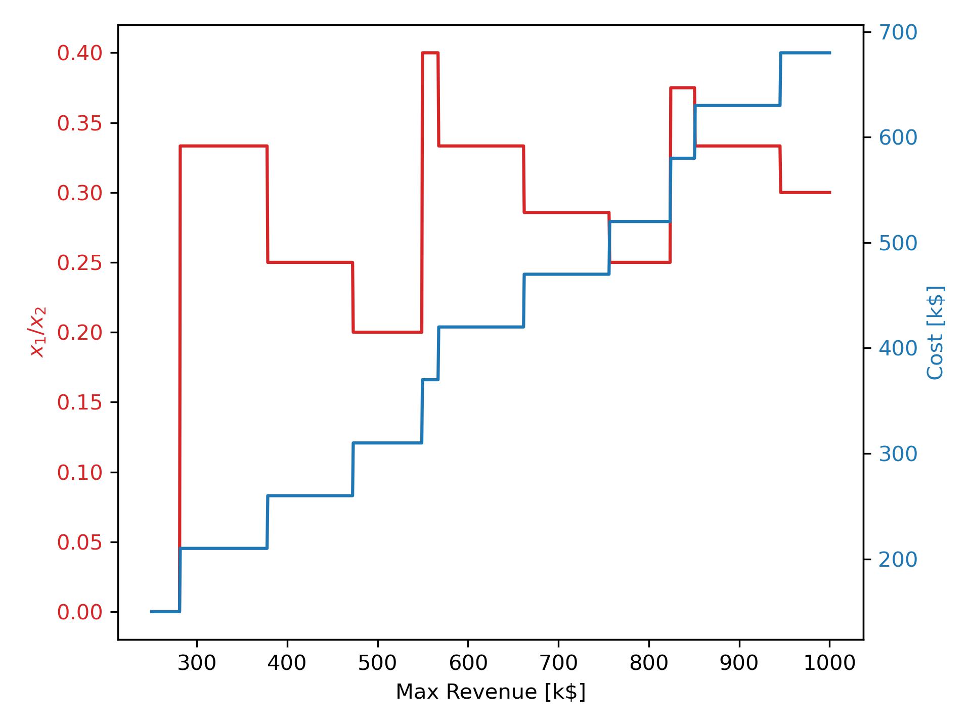
We can ask ourselves, for a given maximum revenue, what would be the ratio between employees from market A, $x_1$, and employees from market B, $x_2$. This can be seen in the figure below, red line and left y-axis.

The chart shows the ratio between the two types of employees for the optimal solution as a function of the maximum revenue (red line and left y-axis), and the corresponding total salary cost also as a function of the office revenue cap (blue line and right y-axis).

After the initial ramp up, we can observe the red line oscillate around a 1 to 3 ratio (~ 0.3), which is consistent with the steps the red line takes (three down and then one up). What the chart shows is that approximately every three employees from market B it becomes convenient to hire an employee from market A.

It’s validating to notice that the rule of thumb just obtained from the $N = 1$ case is compatible with what we observed earlier in the $N = 3$ example (see its outcome above).

Recap

Constrained optimisation is an interesting and rich subject. We looked at what constrained optimisation is and carried out an exercise. We studied the problem from different points of view, we flashed out a Python implementation, and we used the tools developed to improve our understanding of the underlying mathematical model.

“I do the very best I know how—the very best I can; and I mean to keep on doing so until the end. ”—Abraham Lincoln

These type of problems are omnipresent in data science across multiple fields and industries, from hiring departments recruiting new employees to baseball general managers putting together their star team for a new season, and everything in between—including particle physicists extracting standard model parameters from CERN’s LHC data (just saying).